Pytorch是很好的深度学习框架,但在使用时你可能仍然不清楚其中一些概念.这里我只以官方文档为依据尝试解释其中一些概念和方法. 我这里可以称作Effective Pytorch.
update:为了更好的理解pytorch,也许可以从零写点代码karpathy/micrograd: A tiny scalar-valued autograd engine and a neural net library on top of it with PyTorch-like API (github.com)
tensor
Tensor
pytorch默认浮点类型是torch.float32,可以使用torch.set_default_dtype修改
torch.zeros等默认类型就是就是torch.float32,使用torch.set_default_dtype修改默认类型.
torch.tensor() 总是复制data(深拷贝,表示地址不相同).如果你有一个张量数据,只是想更改它的 requiresgrad 标志,请使用 requires_grad() 或 detach() 来避免复制.
如果你有一个 numpy 数组,并希望避免复制,请使用 torch.as_tensor().1
2
3
4
5
6
7torch.device('cuda:0')
torch.device('cpu')
torch.device('mps')
torch.device('cuda') # current cuda device1
2
3
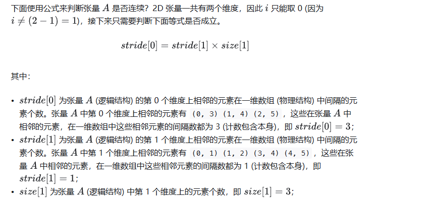
4x = torch.tensor([[1, 2, 3, 4, 5], [6, 7, 8, 9, 10]])
x.stride() #(5,1)
x.t().stride() #(1,5)
Views
PyTorch 允许张量成为现有张量的 “views”.视图张量与其基础张量共享相同的底层数据.支持 “views “可以避免显式数据复制,从而使我们能够进行快速、高效的内存重塑、切片和元素操作.1
2
3
4
5t = torch.rand(4, 4)
b = t.view(2, 8)
t.storage().data_ptr() == b.storage().data_ptr() # `t` and `b` share the same underlying data.
b[0][0] = 3.14
t[0][0]
由于views与其基础张量共享底层数据,因此如果修改views中的数据,也会反映在基础张量中.
通常,PyTorch 操作会返回一个新的张量作为输出,例如 add().但在视图操作中,输出是输入张量的视图,以避免不必要的数据复制.创建视图时不会发生数据移动,视图张量只是改变了解释相同数据的方式.
对连续张量进行视图处理可能会产生非连续张量.transpose() 就是一个常见的例子.(包括view,transpose等操作都会返回view,也就是数据存储与输入相同)1
2
3
4
5base = torch.tensor([[0, 1],[2, 3]])
base.is_contiguous()
t = base.transpose(0, 1) # `t` is a view of `base`. No data movement happened here.
t.is_contiguous()
c = t.contiguous()
Extending PyTorch
原文Extending PyTorch — PyTorch 2.3 documentation
extending torch.autograd
为 autograd 添加操作需要为每个操作实现一个新的 Function 子类.
如何使用
一般来说,如果想在模型中执行不可微分的计算或依赖非 PyTorch 库(如 NumPy),但仍希望您的操作能与其他操作连锁并与 autograd 引擎一起工作,那么请使用自定义函数.
在某些情况下,也可以使用自定义函数来提高性能和内存使用率: 如果您使用 C++ 扩展实现了前向和后向传递,您可以将它们封装在 Function 中,以便与 autograd 引擎对接.如果您想减少为后向传递保存的缓冲区数量,可以使用自定义函数将操作组合在一起.
如果想在后向传递过程中改变梯度或执行副作用,可以考虑register一个张量或模块hook
什么时候不用
如果已经可以用 PyTorch 的内置操作来编写函数,那么它的反向图(很可能)已经可以被 autograd 记录下来.在这种情况下,不需要自己实现后向函数.可以考虑使用一个普通的 Python 函数。
如果需要维护状态,即可训练参数,则应(也可以)使用自定义模块torch.nn.
如果想在后向传递过程中改变梯度或执行副作用,可以考虑注册一个张量或模块钩子。
注意,我在看pytorch2.3时 register_backward_hook已经deprecated了,使用register_full_backward_hook
使用一个register_full_backward_hook将梯度变为相反数.
hook(module, grad_input, grad_output) -> tuple(Tensor) 或 None
grad_input 和 grad_output 是元组,分别包含相对于输入和输出的梯度。钩子不应修改其参数,但可以选择返回一个新的相对于输入的梯度,该梯度将在后续计算中代替 grad_input.对于所有非张量参数,grad_input 和 grad_output 中的条目均为 “None”.
如果想在后向传递过程中改变梯度或执行副作用,可以考虑注册一个张量或模块钩子.1
2
3
4
5
6
7
8
9
10
11def backward_hook(module, grad_input, grad_output):
output_grad_input = - grad_input[0]
return (output_grad_input,)
class negGradient(nn.Module):
def __init__(self):
super(negGradient, self).__init__()
self.register_full_backward_hook(backward_hook)
def forward(self, x):
return x
在domain adaptation的早期论文比如DANN中,一般会使用Function进行梯度变为负数,其实也可以注册backward的hook实现.1
2
3
4
5
6
7
8
9
10
11
12
13
14
15
16
17
18
19class _GradReverseLayer(Function):
def forward(ctx, x, constant):
assert isinstance(constant, int) and constant > 0
ctx.constant = constant
return x.view_as(x)
def backward(ctx, grad_output):
return grad_output.neg() * ctx.constant, None
class GradReverseLayer(nn.Module):
def __init__(self, weight):
super(GradReverseLayer, self).__init__()
self.weight = weight
def forward(self, x):
return _GradReverseLayer.apply(x, self.weight)
既然介绍了register_full_backward_hook,再说说register_forward_hook,每次 forward() 计算完输出后,都会调用该钩子。如果 with_kwargs 为 False 或未指定,输入将只包含给模块的位置参数。关键字参数不会传递给钩子,只会传递给 forward。钩子可以修改输出.钩子可以就地修改输入,但不会对 forward 产生影响,因为钩子是在调用 forward() 之后才调用的.
可以看看这篇文章深入理解PyTorch中的Hook机制:特征可视化的重要工具与实践-CSDN博客
使用方法
采取以下步骤 1. 继承类 Function 并实现 forward()、(可选)setup_context() 和 backward() 方法。2. 在 ctx 参数上调用适当的方法。3. 声明您的函数是否支持 double backward。4. 使用 gradcheck 验证梯度是否正确。
step1:
- forward() 是执行操作的代码。它可以接受任意多个参数,如果指定默认值,其中一些参数是可选的.在调用之前,跟踪历史的张量参数(即 requires_grad=True)将被转换为不跟踪历史的参数,它们的使用将被记录在图中。请注意,此逻辑不会遍历列表/数据集/任何其他数据结构,只会考虑作为调用直接参数的张量.您可以返回一个张量输出,如果有多个输出,也可以返回一个张量元组。
- setup_context()(可选)。可以编写一个接受 ctx 对象的 “组合 “forward(),或者(从 PyTorch 2.0 开始)编写一个不接受 ctx 的单独 forward(),以及一个用于修改 ctx 的 setup_context()方法。forward() 应该具有计算功能,而 setup_context() 应该只负责修改 ctx(而不具有任何计算功能)。一般来说,独立的 forward() 和 setup_context()更接近 PyTorch 本机操作的工作方式,因此更容易与各种 PyTorch 子系统兼容。
- backward()(或 vjp())定义梯度公式。输出有多少个张量参数,它就有多少个张量参数,每个张量参数都代表该输出的梯度。切勿就地修改这些参数。它应该返回与输入相同数量的张量,其中每个张量都包含对应输入的梯度。如果输入不需要梯度(needs_input_grad 是一个布尔元组,表示每个输入是否需要梯度计算),或者是非张量对象,则可以返回 python:None。此外,如果 forward() 的参数是可选的,只要它们都是 None,返回的梯度值就会多于输入值。
1 | class Exp(Function): |
step 2:正确使用 ctx 中的函数,以确保新函数在 autograd 引擎中正常工作。
ctx上有许多方法可用于调用,比较多的就是save_for_backward
必须使用 save_for_backward()来保存要在后向传递中使用的张量。非张量应直接保存在 ctx 上。如果既不是输入也不是输出的张量被保存,那函数函数可能不支持double backward 。
此外还有set_materialize_grads
set_materialize_grads()可以用来告诉 autograd 引擎,在输出不依赖于输入的情况下,通过不对后向函数中的梯度张量进行实体化来优化梯度计算。
step3:如果函数不支持double backward ,则应通过使用 once_differentiable() 对逆运算进行装饰来明确声明这一点。使用此装饰器后,通过函数执行double backward 的尝试将产生错误。1
torch.autograd.gradcheck(Exp.apply, x)
step4:建议使用 torch.autograd.gradcheck() 检查后向函数是否能正确计算前向梯度,方法是使用后向函数计算雅各布矩阵,并将该值与使用有限差分法数值计算的雅各布值进行逐元素比较。1
2
3
4
5
6
7
8
9
10
11
12
13
14
15
16
17
18
19
20
21
22
23
24
25
26
27
28
29
30
31
32
33
34
35
36
37
38
39
40
41# Inherit from Function
class LinearFunction(Function):
# Note that forward, setup_context, and backward are @staticmethods
def forward(input, weight, bias):
output = input.mm(weight.t())
if bias is not None:
output += bias.unsqueeze(0).expand_as(output)
return output
# inputs is a Tuple of all of the inputs passed to forward.
# output is the output of the forward().
def setup_context(ctx, inputs, output):
input, weight, bias = inputs
ctx.save_for_backward(input, weight, bias)
# This function has only a single output, so it gets only one gradient
def backward(ctx, grad_output):
# This is a pattern that is very convenient - at the top of backward
# unpack saved_tensors and initialize all gradients w.r.t. inputs to
# None. Thanks to the fact that additional trailing Nones are
# ignored, the return statement is simple even when the function has
# optional inputs.
input, weight, bias = ctx.saved_tensors
grad_input = grad_weight = grad_bias = None
# These needs_input_grad checks are optional and there only to
# improve efficiency. If you want to make your code simpler, you can
# skip them. Returning gradients for inputs that don't require it is
# not an error.
if ctx.needs_input_grad[0]:
grad_input = grad_output.mm(weight)
if ctx.needs_input_grad[1]:
grad_weight = grad_output.t().mm(input)
if bias is not None and ctx.needs_input_grad[2]:
grad_bias = grad_output.sum(0)
return grad_input, grad_weight, grad_bias
上面这个例子已经写得很好了.为了更方便地使用这些自定义操作,建议将它们别名或封装在一个函数中。使用函数封装可以让我们支持默认参数和关键字参数1
2
3
4
5
6# Option 1: alias
linear = LinearFunction.apply
# Option 2: wrap in a function, to support default args and keyword args.
def linear(input, weight, bias=None):
return LinearFunction.apply(input, weight, bias)
此外还有输入没有tensor的情况,1
2
3
4
5
6
7
8
9
10
11
12
13
14
15
16
17
18
19
20
21
22
23
24
25
26
27
28
29
30
31
32
33
34
35
36
37
38
39
40
41class MulConstant(Function):
def forward(tensor, constant):
return tensor * constant
def setup_context(ctx, inputs, output):
# ctx is a context object that can be used to stash information
# for backward computation
tensor, constant = inputs
ctx.constant = constant # 注意这里直接使用ctx.xx = xx
def backward(ctx, grad_output):
# We return as many input gradients as there were arguments.
# Gradients of non-Tensor arguments to forward must be None.
return grad_output * ctx.constant, None
# 上面代码可以改为 使用set_materialize_grads,因为计算梯度不需要tensor.
class MulConstant(Function):
def forward(tensor, constant):
return tensor * constant
def setup_context(ctx, inputs, output):
tensor, constant = inputs
ctx.set_materialize_grads(False)
ctx.constant = constant
def backward(ctx, grad_output):
# Here we must handle None grad_output tensor. In this case we
# can skip unnecessary computations and just return None.
if grad_output is None:
return None, None
# We return as many input gradients as there were arguments.
# Gradients of non-Tensor arguments to forward must be None.
return grad_output * ctx.constant, None
如果需要保存在 forward() 中计算的任何 “中间 “张量,必须将它们作为输出返回,或者将 forward 和 setup_context()合并.1
2
3
4
5
6
7
8
9
10
11
12
13
14
15
16
17
18
19
20
21
22
23
24
25
26
27
28class MyCube(torch.autograd.Function):
def forward(x):
# We wish to save dx for backward. In order to do so, it must
# be returned as an output.
dx = 3 * x ** 2
result = x ** 3
return result, dx
def setup_context(ctx, inputs, output):
x, = inputs
result, dx = output
ctx.save_for_backward(x, dx)
def backward(ctx, grad_output, grad_dx):
x, dx = ctx.saved_tensors
# In order for the autograd.Function to work with higher-order
# gradients, we must add the gradient contribution of `dx`,
# which is grad_dx * 6 * x.
result = grad_output * dx + grad_dx * 6 * x
return result
# Wrap MyCube in a function so that it is clearer what the output is
def my_cube(x):
result, dx = MyCube.apply(x)
return result
将forward和setup_context合在一起1
2
3
4
5
6
7
8
9
10
11
12
13
14
15
16
17
18
19
20
21
22
23
24class LinearFunction(Function):
# ctx is the first argument to forward
def forward(ctx, input, weight, bias=None):
# The forward pass can use ctx.
ctx.save_for_backward(input, weight, bias)
output = input.mm(weight.t())
if bias is not None:
output += bias.unsqueeze(0).expand_as(output)
return output
def backward(ctx, grad_output):
input, weight, bias = ctx.saved_tensors
grad_input = grad_weight = grad_bias = None
if ctx.needs_input_grad[0]:
grad_input = grad_output.mm(weight)
if ctx.needs_input_grad[1]:
grad_weight = grad_output.t().mm(input)
if bias is not None and ctx.needs_input_grad[2]:
grad_bias = grad_output.sum(0)
return grad_input, grad_weight, grad_bias
extending torch.nn
1 | class Linear(nn.Module): |
可以通过定义具有与 Tensor 匹配的方法的自定义类来创建模拟 Tensor 的自定义类型。如果自定义 Python 类型定义了名为__torch_function__的方法,当您的自定义类的实例被传递给 torch 命名空间中的函数时,PyTorch 将调用您的 __torch_function__实现。这使得为 torch 命名空间中的任何函数定义自定义实现成为可能,__torch_function__实现可以调用这些函数,从而允许您的用户在他们已经为 Tensor 编写的现有 PyTorch 工作流中使用您的自定义类型。
这适用于与 Tensor 无关的 “duck “类型以及 Tensor 子类。
Extending torch Tensor-like type
1 | HANDLED_FUNCTIONS = {} |
为 ScalarTensor 添加 __torch_function__ 实现后,上述操作就有可能成功.这次添加一个__torch_function__ 实现1
2
3
4
5
6
7
8
9
10
11
12
13
14
15
16
17
18
19
20
21
22HANDLED_FUNCTIONS = {}
class ScalarTensor(object):
def __init__(self, N, value):
self._N = N
self._value = value
def __repr__(self):
return "ScalarTensor(N={}, value={})".format(self._N, self._value)
def tensor(self):
return self._value * torch.eye(self._N)
def __torch_function__(cls, func, types, args=(), kwargs=None):
if kwargs is None:
kwargs = {}
if func not in HANDLED_FUNCTIONS or not all(
issubclass(t, (torch.Tensor, ScalarTensor))
for t in types
):
return NotImplemented
return HANDLED_FUNCTIONS[func](*args, **kwargs)
__torch_function__方法需要四个参数:func,对要重载的 torch API 函数的引用;types,实现 __torch_function__的 Tensor-likes 类型列表;args,传递给函数的参数元组;kwargs,传递给函数的关键字参数 dict,它使用名为 HANDLED_FUNCTIONS 的全局调度表来存储自定义实现.1
2
3
4
5
6
7
8
9
10
11
12
13
14
15import functools
def implements(torch_function):
"""Register a torch function override for ScalarTensor"""
def decorator(func):
functools.update_wrapper(func, torch_function)
HANDLED_FUNCTIONS[torch_function] = func
return func
return decorator
def mean(input):
return float(input._value) / input._N
d = ScalarTensor(5, 2)
torch.mean(d)
从 1.7.0 版开始,应用于 torch.Tensor 子类的 torch.Tensor 方法和公共 torch.* 命名空间中的函数将返回子类实例,而不是 torch.Tensor 实例.
如果希望对所有张量方法进行全局覆盖,可以使用__torch_function__1
2
3
4
5
6
7
8
9class LoggingTensor(torch.Tensor):
def __torch_function__(cls, func, types, args=(), kwargs=None):
# NOTE: Logging calls Tensor.__repr__, so we can't log __repr__ without infinite recursion
if func is not torch.Tensor.__repr__:
logging.info(f"func: {func.__name__}, args: {args!r}, kwargs: {kwargs!r}")
if kwargs is None:
kwargs = {}
return super().__torch_function__(func, types, args, kwargs)
在子类的__torch_function__ 中应注意始终调用 super().torch_function(func,…),而不是直接调用 func。如果不这样做,可能会导致 func 返回到 __torch_function__中,从而引起无限递归。
torch.autograd
torch.autograd 提供了实现任意标量值函数自动微分的类和函数.
它只需对现有代码做极少的改动—你只需用 requires_grad=True 关键字声明需要计算梯度的张量.
目前只持浮点张量类型(半浮点、浮点、双浮点和 bfloat16)和复合张量类型(cfloat、cdouble)的 autograd.
detach 计算图与leaf tensor
Tensor.detach()返回一个从当前计算图中分离出来的新张量,生成的张量永远不需要梯度,目前替代了.data方法.
PyTorch 中,计算图(Computation Graph)是一个非常重要的概念.它是一种用于表示和执行机器学习模型的数据结构.
具体来说,PyTorch 中的计算图由以下几个关键组件组成:
- 张量(Tensor):计算图的基本单元,表示输入数据、中间结果和最终输出.
- 操作(Operation):在张量上执行的各种数学运算,如加法、乘法、卷积等.
- 节点(Node):表示张量和操作,计算图由这些节点组成.
- 边(Edge):表示节点之间的依赖关系,数据沿着边流动.
当在 PyTorch 中定义和执行机器学习模型时,PyTorch 会自动构建一个计算图来表示模型的结构和数据流.这个计算图可以用于以下几个方面:
- 前向传播:通过计算图,PyTorch 可以自动计算模型的输出.
- 反向传播:当您调用
loss.backward()时,PyTorch 会沿着计算图反向传播梯度,从而更新模型参数. - 可视化:您可以使用 PyTorch 提供的工具(如 TensorBoard)来可视化计算图,更好地理解模型的结构.
- 优化:PyTorch 的优化器会利用计算图的结构来提高优化效率.
detach使得tensor从计算图中分离具体是什么含义?简单来说,使得它本身requires_grad=False,它之前的计算也被阻断了.1
2
3
4
5
6
7
8input = torch.randn(1, 20, 10)
model = nn.Linear(10, 3)
inter = model(input)
model2 = nn.Linear(3, 1)
output = model2(inter.detach())
loss = torch.mean(output - 1)
loss.backward()
print(model.weight.grad) # None
按照惯例,所有requires_grad 为False的张量都是leaf tensor.
对于requires_grad 为 True 的张量,如果它们是由用户创建(没有经过计算,包括移动到GPU的操作)的,那么它们将是叶子张量.这意味着它们不是操作的结果,因此 grad_fn 为 None.
只有叶子张量才会在调用 backward() 时被填充梯度.要为非叶子张量填充阶值,可以使用 retain_grad().1
2
3
4
5
6
7
8
9
10xx = torch.randn(1, 3).requires_grad_(True)
print(xx.grad_fn, xx.is_leaf) # None,True
model = nn.Linear(3, 1)
output = model(xx)
loss = torch.mean(output - 1)
loss.backward()
print(xx.grad_fn, xx.grad) # None,tensor([[.., .., ..]])
print(model.weight.grad_fn, model.weight.grad) # None,,tensor([[.., .., ..]])
print(model.bias.grad_fn, model.bias.grad) # None,tensor([1])
print(model.weight.is_leaf, model.bias.is_leaf) # True,True
只能获取计算图中叶子节点的梯度属性,这些节点的 requires_grad 属性设置为 True.对于图中的所有其他节点,梯度属性将不可用.
出于性能考虑,我们只能在给定图形上使用一次后向操作执行梯度计算.如果我们需要在同一图形上执行多次 backward 调用,则需要向 backward 调用传递 retain_graph=True 属性.
几个问题:
leaf tensor的grad_fn一定为空吗? 不一定,用户创建的requires_grad为True的tensor的grad_fn不为空
leaf tensor一定是模型输入吗?不一定,事实上直接创建一个模型,它的weight和bias也是leaf tensor
属于旧时代的Variable和data
Variable API 已被弃用:使用张量时,不再需要Variable.如果 requires_grad 设置为 True,Autograd 将自动支持张量.
Variable(tensor) 和 Variable(tensor, requires_grad) 仍按预期工作,但它们返回的是张量而不是变量.
var.data 与 tensor.data 相同.
var.backward()、var.detach()、var.register_hook() 等方法现在可以在具有相同方法名的张量上运行.
此外,现在还可以使用 torch.randn()、torch.zeros()、torch.none() 等工厂方法创建 requires_grad=True 的张量:1
autograd_tensor = torch.randn((2, 3, 4), requires_grad=True)
| api | 介绍 |
|---|---|
torch.Tensor.grad | This attribute is None by default and becomes a Tensor the first time a call to backward() computes gradients for self |
torch.Tensor.requires_grad | Is True if gradients need to be computed for this Tensor, False otherwise. |
torch.Tensor.is_leaf | All Tensors that have requires_grad which is False will be leaf Tensors by convention. |
torch.Tensor.backward([gradient, …]) | Computes the gradient of current tensor wrt graph leaves. |
torch.Tensor.detach | Returns a new Tensor, detached from the current graph. |
torch.Tensor.detach_ | Detaches the Tensor from the graph that created it, making it a leaf. |
torch.Tensor.register_hook(hook) | Registers a backward hook. |
torch.Tensor.register_post_accumulate_grad_hook(hook) | Registers a backward hook that runs after grad accumulation. |
torch.Tensor.retain_grad() | Enables this Tensor to have their grad populated during backward(). |
Function
要创建自定义 autograd.Function,请继承该类并实现 forward() 和 backward() 静态方法.然后,要在前向传递中使用自定义 op,调用类方法 apply.不要直接调用 forward().1
2
3
4
5
6
7
8
9
10
11
12
13class Exp(Function):
def forward(ctx, i):
result = i.exp()
ctx.save_for_backward(result)
return result
def backward(ctx, grad_output):
result, = ctx.saved_tensors
return grad_output * result
Use it by calling the apply method:
output = Exp.apply(input)
ONNX格式
在实际部署时非常常用的模型格式,是屏蔽了框架的.
保存模型
1 | import torch |
生成的 alexnet.onnx 文件包含一个 protocol buffer,其中包含了导出的模型(在本例中为 AlexNet)的网络结构和参数.verbose=True 参数会导致导出器打印出模型的人类可读表示.
加载模型
1 | pip install onnx |
1 | import onnx |
流程
1 | # Input to the model |
在pytorch中直接使用torch.onnx.export即可.
因为导出运行了模型,我们需要提供一个输入张量 x.这个输入的值可以是随机的,只要它的类型和大小是正确的.请注意,除非指定为dynamic_axes,否则导出的 ONNX 图中输入的所有维度大小都会被固定下来.在这个示例中,使用批量大小为 1 的输入导出模型,但在 torch.onnx.export() 的 dynamic_axes 参数中指定了第一个维度为动态的.因此,导出的模型将接受大小为 [batch_size, 1, 224, 224] 的输入,其中 batch_size 可以是可变的.
同时还计算了模型输出 torch_out,我们将使用它来验证在 ONNX Runtime 中运行时导出的模型是否计算出相同的值.
但在使用 ONNX Runtime 验证模型输出之前,我们会先使用 ONNX API 检查 ONNX 模型.首先,onnx.load("super_resolution.onnx") 会加载保存的模型,并输出一个 onnx.ModelProto 结构.然后,onnx.checker.check_model(onnx_model) 会验证模型的结构,并确认模型具有有效的架构.通过检查模型的版本、图结构以及节点及其输入和输出,来验证 ONNX 图的有效性.1
2
3import onnx
onnx_model = onnx.load("super_resolution.onnx")
onnx.checker.check_model(onnx_model)
使用 ONNX Runtime 的 Python API 计算输出,通常情况下,这一部分可以在单独的进程中或其他机器上完成,但我们将继续在同一进程中进行,这样我们就可以验证 ONNX Runtime 和 PyTorch 为该网络计算出的值是否相同.
为了使用 ONNX Runtime 运行模型,我们需要为模型创建一个InferenceSession,并设置所需的配置参数(这里我们使用默认配置).创建会话后,我们就可以使用 run() API 来评估模型了.该调用的输出是一个列表,包含 ONNX Runtime 计算得出的模型输出.1
2
3
4
5
6
7
8
9
10
11
12
13
14
15import onnxruntime
ort_session = onnxruntime.InferenceSession("super_resolution.onnx", providers=["CPUExecutionProvider"])
def to_numpy(tensor):
return tensor.detach().cpu().numpy() if tensor.requires_grad else tensor.cpu().numpy()
# compute ONNX Runtime output prediction
ort_inputs = {ort_session.get_inputs()[0].name: to_numpy(x)}
ort_outs = ort_session.run(None, ort_inputs)
# compare ONNX Runtime and PyTorch results
np.testing.assert_allclose(to_numpy(torch_out), ort_outs[0], rtol=1e-03, atol=1e-05)
print("Exported model has been tested with ONNXRuntime, and the result looks good!")
注意
在模型中避免使用numpy,tensor.data,tensor.shape不能使用in_place操作
自动混合精度
torch.amp 为混合精度提供了方便的方法,其中一些操作使用 torch.float32 (浮点)数据类型,另一些操作使用较低精度的浮点数据类型 (lower_precision_fp):torch.float16(半精度)或 torch.bfloat16.一些操作,如线性层和卷积,在 lower_precision_fp 下速度更快.其他操作,如还原,通常需要 float32 的动态范围.混合精度试图将每个操作与相应的数据类型相匹配.
通常,数据类型为 torch.float16 的 “自动混合精度训练 “使用 torch.autocast 和 torch.cpu.amp.GradScaler 或 torch.cuda.amp.GradScaler.
torch.autocast 实例可对所选上下文进行自动casting.自动cast会自动选择 GPU 运算的精度,从而在保持精度的同时提高性能.
torch.cuda.amp.GradScaler 的实例有助于方便地执行梯度缩放步骤.梯度缩放可最大限度地减少梯度下溢,从而改善具有 float16 梯度的网络的收敛性.1
2
3
4
5
6
7
8
9
10
11
12
13
14
15
16
17
18
19
20
21
22
23
24
25
26
27
28# Creates model and optimizer in default precision
model = Net().cuda()
optimizer = optim.SGD(model.parameters(), ...)
# Creates a GradScaler once at the beginning of training.
scaler = GradScaler() # 1. 创建gradscaler
for epoch in epochs:
for input, target in data:
optimizer.zero_grad()
# Runs the forward pass with autocasting.
# 2.使得模型训练时相关参数类型自动转换
with autocast(device_type='cuda', dtype=torch.float16):
output = model(input)
loss = loss_fn(output, target)
# Scales loss. Calls backward() on scaled loss to create scaled gradients.
# Backward passes under autocast are not recommended.
# Backward ops run in the same dtype autocast chose for corresponding forward ops.
scaler.scale(loss).backward()
# scaler.step() first unscales the gradients of the optimizer's assigned params.
# If these gradients do not contain infs or NaNs, optimizer.step() is then called,
# otherwise, optimizer.step() is skipped.
scaler.step(optimizer)
# Updates the scale for next iteration.
scaler.update()1
2
3
4
5
6
7
8
9
10
11
12
13
14
15# Creates model and optimizer in default precision
model = Net().cuda()
optimizer = optim.SGD(model.parameters(), ...)
for input, target in data:
optimizer.zero_grad()
# Enables autocasting for the forward pass (model + loss)
with torch.autocast(device_type="cuda"):
output = model(input)
loss = loss_fn(output, target)
# Exits the context manager before backward()
loss.backward()
optimizer.step()
所有由 scaler.scale(loss).backward() 生成的梯度都是按比例缩放的.如果要在 backward() 和 scaler.step(optimizer) 之间修改或检查参数的 .grad 属性,应首先取消缩放.
梯度惩罚
梯度惩罚的实现通常使用 torch.autograd.grad() 创建梯度,将它们组合起来创建惩罚值,并将惩罚值添加到损失中.1
2
3
4
5
6
7
8
9
10
11
12
13
14
15
16
17
18
19
20
21
22
23for epoch in epochs:
for input, target in data:
optimizer.zero_grad()
output = model(input)
loss = loss_fn(output, target)
# Creates gradients
grad_params = torch.autograd.grad(outputs=loss,
inputs=model.parameters(),
create_graph=True)
# Computes the penalty term and adds it to the loss
grad_norm = 0
for grad in grad_params:
grad_norm += grad.pow(2).sum()
grad_norm = grad_norm.sqrt()
loss = loss + grad_norm
loss.backward()
# clip gradients here, if desired
optimizer.step()
要通过梯度缩放实现梯度惩罚,应缩放传递给 torch.autograd.grad() 的输出张量.因此,生成的梯度也将被缩放,在合并生成惩罚值之前应取消缩放.
此外,惩罚项的计算是前向传递的一部分,因此应在自动传递上下文中进行.1
2
3
4
5
6
7
8
9
10
11
12
13
14
15
16
17
18
19
20
21
22
23
24
25scaler = torch.cuda.amp.GradScaler()
for epoch in epochs:
for input, target in data:
optimizer0.zero_grad()
optimizer1.zero_grad()
with autocast(device_type='cuda', dtype=torch.float16):
output0 = model0(input)
output1 = model1(input)
loss0 = loss_fn(2 * output0 + 3 * output1, target)
loss1 = loss_fn(3 * output0 - 5 * output1, target)
# (retain_graph here is unrelated to amp, it's present because in this
# example, both backward() calls share some sections of graph.)
scaler.scale(loss0).backward(retain_graph=True)
scaler.scale(loss1).backward()
# You can choose which optimizers receive explicit unscaling, if you
# want to inspect or modify the gradients of the params they own.
scaler.unscale_(optimizer0)
scaler.step(optimizer0)
scaler.step(optimizer1)
scaler.update()
如果网络有多个损失,则必须对每个损耗单独调用 scaler.scale.如果的网络有多个优化器,您可以在任何一个优化器上单独调用 scaler.unscale_,并且必须在每个优化器上单独调用 scaler.step.
autocast不在在 float64 或非浮点类型上进行转换.。为了获得最佳性能和稳定性,在autocast区域中使用out-of-place运算,也就是使用类似a.addmm(b, c)这种操作.
autocast会将with下的区域中的运算自动转换,自动转发应只包含网络的前向传递,包括损失计算。
不建议使用自动转发的后向传递. 后向操作的运算类型是autocast之前的类型.
cuda上会转为float16的运算
1 | __matmul__`, `addbmm`, `addmm`, `addmv`, `addr`, `baddbmm`, `bmm`, `chain_matmul`, `multi_dot`, `conv1d`, `conv2d`, `conv3d`, `conv_transpose1d`, `conv_transpose2d`, `conv_transpose3d`, `GRUCell`, `linear`, `LSTMCell`, `matmul`, `mm`, `mv`, `prelu`, `RNNCell |
cuda上会转为float32的运算
1 | __pow__`, `__rdiv__`, `__rpow__`, `__rtruediv__`, `acos`, `asin`, `binary_cross_entropy_with_logits`, `cosh`, `cosine_embedding_loss`, `cdist`, `cosine_similarity`, `cross_entropy`, `cumprod`, `cumsum`, `dist`, `erfinv`, `exp`, `expm1`, `group_norm`, `hinge_embedding_loss`, `kl_div`, `l1_loss`, `layer_norm`, `log`, `log_softmax`, `log10`, `log1p`, `log2`, `margin_ranking_loss`, `mse_loss`, `multilabel_margin_loss`, `multi_margin_loss`, `nll_loss`, `norm`, `normalize`, `pdist`, `poisson_nll_loss`, `pow`, `prod`, `reciprocal`, `rsqrt`, `sinh`, `smooth_l1_loss`, `soft_margin_loss`, `softmax`, `softmin`, `softplus`, `sum`, `renorm`, `tan`, `triplet_margin_loss |
还有一些运算需要多个输入,如果输入全是float32那输出就是float32.也就是promote to the widest input type1
addcdiv`, `addcmul`, `atan2`, `bilinear`, `cross`, `dot`, `grid_sample`, `index_put`, `scatter_add`, `tensordot
CPU上会转为bfloat16的运算
bfloat是比较特殊的数据类型,是针对深度学习运算特别调整指数位和小数位,使得相对于同等位数的float,其精度更小,但能表示的值范围更大,而且针对显卡运算更快(显卡厂商调整了)
| Format | Bits | Exponent | Fraction | sign(符号) |
|---|---|---|---|---|
| FP32 | 32 | 8 | 23 | 1 |
| FP16 | 16 | 5 | 10 | 1 |
| BF16 | 16 | 8 | 7 | 1 |
1 | conv1d`, `conv2d`, `conv3d`, `bmm`, `mm`, `baddbmm`, `addmm`, `addbmm`, `linear`, `matmul`, `_convolution |
CPU上会转为bfloat32的运算
1 | conv_transpose1d, conv_transpose2d, conv_transpose3d, avg_pool3d, binary_cross_entropy, grid_sampler, grid_sampler_2d, _grid_sampler_2d_cpu_fallback, grid_sampler_3d, polar, prod, quantile, nanquantile, stft, cdist, trace, view_as_complex, cholesky, cholesky_inverse, cholesky_solve, inverse, lu_solve, orgqr, inverse, ormqr, pinverse, max_pool3d, max_unpool2d, max_unpool3d, adaptive_avg_pool3d, reflection_pad1d, reflection_pad2d, replication_pad1d, replication_pad2d, replication_pad3d, mse_loss, ctc_loss, kl_div, multilabel_margin_loss, fft_fft, fft_ifft, fft_fft2, fft_ifft2, fft_fftn, fft_ifftn, fft_rfft, fft_irfft, fft_rfft2, fft_irfft2, fft_rfftn, fft_irfftn, fft_hfft, fft_ihfft, linalg_matrix_norm, linalg_cond, linalg_matrix_rank, linalg_solve, linalg_cholesky, linalg_svdvals, linalg_eigvals, linalg_eigvalsh, linalg_inv, linalg_householder_product, linalg_tensorinv, linalg_tensorsolve, fake_quantize_per_tensor_affine, eig, geqrf, lstsq, _lu_with_info, qr, solve, svd, symeig, triangular_solve, fractional_max_pool2d, fractional_max_pool3d, adaptive_max_pool3d, multilabel_margin_loss_forward, linalg_qr, linalg_cholesky_ex, linalg_svd, linalg_eig, linalg_eigh, linalg_lstsq, linalg_inv_ex |
类似的,cpu上也有promote to the widest input type的运算.1
cat, stack, index_copy
单机器(多GPU)训练最佳实践
如果有多个GPU,每个GPU上运行复制的权重相同的模型,数据分发到多个GPU上,这样就能加快训练.但是有些使用一个GPU上容不下一个完整的模型,这个时候,将一个模型拆到不同的GPU上就是一个可行的方案.
这里就要提到model parallel(模型并行),模型并行是将一个模型的不同子网络放到不同的设备上,并相应地forward,以便在设备间移动中间输出.
如果是跨机器,可以通过RPCGetting Started with Distributed RPC Framework — PyTorch Tutorials 2.3.0+cu121 documentation
一个简单的例子1
2
3
4
5
6
7
8
9
10
11
12
13
14
15
16
17
18
19
20
21
22
23
24import torch
import torch.nn as nn
import torch.optim as optim
class ToyModel(nn.Module):
def __init__(self):
super(ToyModel, self).__init__()
self.net1 = torch.nn.Linear(10, 10).to('cuda:0')
self.relu = torch.nn.ReLU()
self.net2 = torch.nn.Linear(10, 5).to('cuda:1')
def forward(self, x):
x = self.relu(self.net1(x.to('cuda:0')))
return self.net2(x.to('cuda:1'))
model = ToyModel()
loss_fn = nn.MSELoss()
optimizer = optim.SGD(model.parameters(), lr=0.001)
optimizer.zero_grad()
outputs = model(torch.randn(20, 10))
labels = torch.randn(20, 5).to('cuda:1')
loss_fn(outputs, labels).backward()
optimizer.step()
把模型不同部分放在了不同GPU上,并且forward时把数据也放在对应位置.注意计算损失时,label也要放对应位置.
只需修改几行代码,就可以在多个 GPU 上运行现有的单 GPU 模块.继承现有的 ResNet 模块,并在构建过程中将各层拆分到两个 GPU.然后,覆盖forward方法,通过相应移动中间输出来缝合两个子网络.1
2
3
4
5
6
7
8
9
10
11
12
13
14
15
16
17
18
19
20
21
22
23
24
25
26
27
28
29
30
31from torchvision.models.resnet import ResNet, Bottleneck
num_classes = 1000
class ModelParallelResNet50(ResNet):
def __init__(self, *args, **kwargs):
super(ModelParallelResNet50, self).__init__(
Bottleneck, [3, 4, 6, 3], num_classes=num_classes, *args, **kwargs)
self.seq1 = nn.Sequential(
self.conv1,
self.bn1,
self.relu,
self.maxpool,
self.layer1,
self.layer2
).to('cuda:0')
self.seq2 = nn.Sequential(
self.layer3,
self.layer4,
self.avgpool,
).to('cuda:1')
self.fc.to('cuda:1')
def forward(self, x):
x = self.seq2(self.seq1(x).to('cuda:1'))
return self.fc(x.view(x.size(0), -1))
最后做了相关实验,发现在多个GPU上模型并行执行时间更长,因为多个 GPU 中只有一个在工作,而其他的也不做,同时数据从不同GPU中复制时也需要时间.

多GPU训练
并行方案
DataParallel是单进程、多线程的,只能在单台机器上(可以多GPU)运行,而 DistributedDataParallel 是多进程的,可以在单台和多台机器上运行.
即使在单台机器上,DataParallel 通常也比 DistributedDataParallel 慢,这是因为线程间的 GIL 竞争、每次迭代的复制模型,以及分散输入和收集输出所带来的额外开销.
实际为了方便,完全可以仅使用DataParaller在多GPU上运行.
| DataParallel | disc |
|---|---|
nn.DataParallel | Implements data parallelism at the module level. |
nn.parallel.DistributedDataParallel | Implement distributed data parallelism based on torch.distributed at module level. |
模型并行:如果模型太大,无法在单个 GPU 上运行,就必须使用模型并行功能将其分割到多个 GPU 上.
分布式数据并行(DistributedDataParallel,DDP)可与模型并行一起使用,而数据并行(DataParallel)目前还不能。当 DDP 与模型并行相结合时,每个 DDP 进程都将使用模型并行,而所有进程都将使用数据并行。
多GPU训练有每个GPU一个线程
torch.nn.DataParallel1
2
3
4
5
6
7
8
9model = MyModel()
dp_model = nn.DataParallel(model)
# Sets autocast in the main thread
with autocast(device_type='cuda', dtype=torch.float16):
# dp_model's internal threads will autocast.
output = dp_model(input)
# loss_fn also autocast
loss = loss_fn(output)
上面方法是最简单的弊端是后续的loss计算只会在cuda:0上进行,没法并行,因此会导致负载不均衡的问题
文档推荐使用DistributedDataParallel
为什么尽管增加了复杂性,还是会考虑使用 DistributedDataParallel 而不是 DataParallel:
首先,DataParallel 是单进程、多线程的,只能在单机上运行,而 DistributedDataParallel 是多进程的,可以在单机和多机训练中运行.即使在单台机器上,DataParallel 通常也比 DistributedDataParallel 慢,这是由于线程间的 GIL 竞争、每次迭代的复制模型,以及分散输入和收集输出所带来的额外开销.
分布式数据并行(DistributedDataParallel)可与模型并行一起使用,而数据并行(DataParallel)目前还不能.当 DDP 与模型并行相结合时,每个 DDP 进程都将使用模型并行,而所有进程都将使用数据并行.
如果模型需要跨越多台机器,或者您的用例不符合数据并行模式,请使用RPC API,以通用的分布式训练.
在模块级基于 torch.distributed 实现分布式数据并行.
该容器通过在每个模型副本之间同步梯度来提供数据并行性.要同步的设备由输入 process_group 指定,默认情况下是整个世界.请注意,DistributedDataParallel 不会在参与的 GPU 之间对输入进行分块或分片;用户负责定义如何进行分块或分片,例如通过使用 DistributedSampler.
此外需要进行初始化 torch.distributed.init_process_group()1
2
3
4
5
6
7
8
9
10
11
12
13
14
15
16
17
18
19
20
21
22
23
24
25
26
27
28
29
30
31
32
33
34
35
36
37
38
39
40
41
42import torch
import torch.distributed as dist
import torch.multiprocessing as mp
import torch.nn as nn
import torch.optim as optim
import os
from torch.nn.parallel import DistributedDataParallel as DDP
def example(rank, world_size):
# create default process group
dist.init_process_group("gloo", rank=rank, world_size=world_size)
# create local model
model = nn.Linear(10, 10).to(rank)
# construct DDP model
ddp_model = DDP(model, device_ids=[rank])
# define loss function and optimizer
loss_fn = nn.MSELoss()
optimizer = optim.SGD(ddp_model.parameters(), lr=0.001)
# forward pass
outputs = ddp_model(torch.randn(20, 10).to(rank))
labels = torch.randn(20, 10).to(rank)
# backward pass
loss_fn(outputs, labels).backward()
# update parameters
optimizer.step()
def main():
world_size = 2
mp.spawn(example,
args=(world_size,),
nprocs=world_size,
join=True)
if __name__=="__main__":
# Environment variables which need to be
# set when using c10d's default "env"
# initialization mode.
os.environ["MASTER_ADDR"] = "localhost"
os.environ["MASTER_PORT"] = "29500"
main() 1
2
3
4
5
6
7
8
9
10
11
12
13
14
15
16
17
18
19
20
21
22
23
24
25
26
27
28
29
30
31def demo_model_parallel(rank, world_size):
print(f"Running DDP with model parallel example on rank {rank}.")
setup(rank, world_size)
# setup mp_model and devices for this process
dev0 = rank * 2
dev1 = rank * 2 + 1
mp_model = ToyMpModel(dev0, dev1)
ddp_mp_model = DDP(mp_model)
loss_fn = nn.MSELoss()
optimizer = optim.SGD(ddp_mp_model.parameters(), lr=0.001)
optimizer.zero_grad()
# outputs will be on dev1
outputs = ddp_mp_model(torch.randn(20, 10))
labels = torch.randn(20, 5).to(dev1)
loss_fn(outputs, labels).backward()
optimizer.step()
cleanup()
if __name__ == "__main__":
n_gpus = torch.cuda.device_count()
assert n_gpus >= 2, f"Requires at least 2 GPUs to run, but got {n_gpus}"
world_size = n_gpus
run_demo(demo_basic, world_size)
run_demo(demo_checkpoint, world_size)
world_size = n_gpus//2
run_demo(demo_model_parallel, world_size)1
2
3
4
5
6
7sampler = DistributedSampler(dataset) if is_distributed else None
loader = DataLoader(dataset, shuffle=(sampler is None),
sampler=sampler)
for epoch in range(start_epoch, n_epochs):
if is_distributed:
sampler.set_epoch(epoch)
train(loader)
它与 torch.nn.parallel.DistributedDataParallel 结合使用尤其有用.在这种情况下,每个进程都可以传递一个 DistributedSampler 实例作为 DataLoader 采样器,并加载其独有的原始数据集子集.1
2
3
4
5
6
7
8
9
10
11
12
13
14
15
16
17
18
19
20
21
22
23
24
25
26
27
28
29
30
31
32
33
34
35
36
37
38
39
40
41
42
43
44
45
46
47
48
49import torch
import torch.distributed as dist
import torch.nn as nn
import torch.optim as optim
from torch.utils.data import DataLoader, Dataset, DistributedSampler
from torch.nn.parallel import DistributedDataParallel as DDP
#### 自定义数据集和模型
class MyDataset(Dataset):
# 实现__len__和__getitem__方法
pass
class MyModel(nn.Module):
# 定义模型结构,可能需要考虑如何拆分模型
pass
#### 初始化分布式环境
dist.init_process_group(backend='nccl', init_method='tcp://localhost:23456', rank=0, world_size=torch.cuda.device_count())
#### 初始化数据集和模型
dataset = MyDataset()
sampler = DistributedSampler(dataset)
dataloader = DataLoader(dataset, batch_size=32, shuffle=False, sampler=sampler)
model = MyModel()
#### 拆分模型(这通常需要根据模型的具体结构来手动完成)
#### 例如,如果模型有两个主要部分,可以将它们分别放到不同的设备上
model_part1 = model.part1.to('cuda:0')
model_part2 = model.part2.to('cuda:1')
#### 使用DistributedDataParallel包装模型
model = DDP(model, device_ids=[torch.cuda.current_device()])
#### 定义损失函数和优化器
criterion = nn.CrossEntropyLoss()
optimizer = optim.Adam(model.parameters(), lr=0.001)
#### 训练循环
for epoch in range(num_epochs):
for inputs, labels in dataloader:
inputs, labels = inputs.to(model.device), labels.to(model.device)
optimizer.zero_grad()
outputs = model(inputs)
loss = criterion(outputs, labels)
loss.backward()
optimizer.step()
#### 销毁分布式进程组
dist.destroy_process_group()
jia-zhuang/pytorch-multi-gpu-training: 整理 pytorch 单机多 GPU 训练方法与原理 (github.com)
常用Container
| Containers | 介绍 |
|---|---|
Module | Base class for all neural network modules. |
Sequential | A sequential container. |
ModuleList | Holds submodules in a list. |
ModuleDict | Holds submodules in a dictionary. |
ParameterList | Holds parameters in a list. |
ParameterDict | Holds parameters in a dictionary. |
Module1
2
3
4
5
6
7
8
9
10
11
12import torch.nn as nn
import torch.nn.functional as F
class Model(nn.Module):
def __init__(self):
super().__init__()
self.conv1 = nn.Conv2d(1, 20, 5)
self.conv2 = nn.Conv2d(20, 20, 5)
def forward(self, x):
x = F.relu(self.conv1(x))
return F.relu(self.conv2(x))
Sequential1
2
3
4
5
6
7
8
9
10
11
12
13
14
15model = nn.Sequential(
nn.Conv2d(1,20,5),
nn.ReLU(),
nn.Conv2d(20,64,5),
nn.ReLU()
)
# Using Sequential with OrderedDict. This is functionally the
# same as the above code
model = nn.Sequential(OrderedDict([
('conv1', nn.Conv2d(1,20,5)),
('relu1', nn.ReLU()),
('conv2', nn.Conv2d(20,64,5)),
('relu2', nn.ReLU())
]))
ModuleList1
2
3
4
5
6
7
8
9
10class MyModule(nn.Module):
def __init__(self):
super().__init__()
self.linears = nn.ModuleList([nn.Linear(10, 10) for i in range(10)])
def forward(self, x):
# ModuleList can act as an iterable, or be indexed using ints
for i, l in enumerate(self.linears):
x = self.linears[i // 2](x) + l(x)
return x
ModuleDict1
2
3
4
5
6
7
8
9
10
11
12
13
14
15
16class MyModule(nn.Module):
def __init__(self):
super().__init__()
self.choices = nn.ModuleDict({
'conv': nn.Conv2d(10, 10, 3),
'pool': nn.MaxPool2d(3)
})
self.activations = nn.ModuleDict([
['lrelu', nn.LeakyReLU()],
['prelu', nn.PReLU()]
])
def forward(self, x, choice, act):
x = self.choices[choice](x)
x = self.activations[act](x)
return x
ParameterList1
2
3
4
5
6
7
8
9
10class MyModule(nn.Module):
def __init__(self):
super().__init__()
self.params = nn.ParameterList([nn.Parameter(torch.randn(10, 10)) for i in range(10)])
def forward(self, x):
# ParameterList can act as an iterable, or be indexed using ints
for i, p in enumerate(self.params):
x = self.params[i // 2].mm(x) + p.mm(x)
return x
ParameterDict1
2
3
4
5
6
7
8
9
10
11class MyModule(nn.Module):
def __init__(self):
super().__init__()
self.params = nn.ParameterDict({
'left': nn.Parameter(torch.randn(5, 10)),
'right': nn.Parameter(torch.randn(5, 10))
})
def forward(self, x, choice):
x = self.params[choice].mm(x)
return x
容易混淆和遗忘的方法
torch.Tensor.scatter_
torch.scatter的in-place操作
Tensor.scatter_(dim, index, src, *, reduce=None) → [Tensor]
按照 index 张量中指定的索引,将张量 src 中的所有值写入 self 中.
对于 src 中的每个值,其输出索引在 dimension != dim 时由 src 中的索引指定,在 dimension = dim 时由 index 中的相应值指定.1
2
3self[index[i][j][k]][j][k] = src[i][j][k] # if dim == 0
self[i][index[i][j][k]][k] = src[i][j][k] # if dim == 1
self[i][j][index[i][j][k]] = src[i][j][k] # if dim == 2
self、index 和 src(如果是张量)的维数应该相同.对于所有维度d,index.size(d) <= src.size(d);对于所有维度 d != dim,index.size(d) <= self.size(d),index 和 src 不会广播.
与gather逆操作,常用作写one-hot量1
2
3
4
5
6
7
8
9
10
11
12
13
14
15index = torch.tensor([[0, 1]])
value = 2
torch.zeros(3, 5).scatter_(0, index, value)
src = torch.arange(1, 11).reshape((2, 5))
src
index = torch.tensor([[0, 1, 2, 0]])
torch.zeros(3, 5, dtype=src.dtype).scatter_(0, index, src)
index = torch.tensor([[0, 1, 2], [0, 1, 4]])
torch.zeros(3, 5, dtype=src.dtype).scatter_(1, index, src)
torch.full((2, 4), 2.).scatter_(1, torch.tensor([[2], [3]]),
1.23, reduce='multiply')
torch.full((2, 4), 2.).scatter_(1, torch.tensor([[2], [3]]),
1.23, reduce='add')
torch.gather
torch.gather(input, dim, index, *, sparse_grad=False, out=None) → [Tensor](https://pytorch.org/docs/stable/tensors.html#torch.Tensor)
输入和索引的维数必须相同. 在 d != dim的维度 中,index.size(d) <= input.size(d)。输入和index不会相互广播1
2
3out[i][j][k] = input[index[i][j][k]][j][k] # if dim == 0
out[i][j][k] = input[i][index[i][j][k]][k] # if dim == 1
out[i][j][k] = input[i][j][index[i][j][k]] # if dim == 21
2t = torch.tensor([[1, 2], [3, 4]])
torch.gather(t, 1, torch.tensor([[0, 0], [1, 0]]))
上面的代码就是把t根据index torch.tensor([[0, 0], [1, 0]])重新得到一个tensor.
scatter是通过index将src的数据放在input中
gather是通过index将input的数据取出来
torch.split
torch.split(tensor, split_size_or_sections, dim=0
将张量分割成块.每个块都是原始张量的一个view.
如果 split_size_or_sections 是整数类型,那么张量将被分割成大小相等的块(如果可能).如果张量在给定维度 dim 上的大小不能被 split_size 整除,则最后一个块的大小会变小.
如果 split_size_or_sections 是一个列表,那么张量将被分割成 len(split_size_or_sections)小块,其大小与 split_size_or_sections 一致.1
2
3
4
5
6
7
8
9
10
11
12
13a = torch.arange(10).reshape(5, 2)
torch.split(a, 2)
(tensor([[0, 1],
[2, 3]]),
tensor([[4, 5],
[6, 7]]),
tensor([[8, 9]]))
torch.split(a, [1, 4])
(tensor([[0, 1]]),
tensor([[2, 3],
[4, 5],
[6, 7],
[8, 9]]))
torch.tensor_split
torch.tensor_split(input, indices_or_sections, dim=0) → List of Tensors
根据 indices_or_sections 指定的索引或部分数,将张量沿维度 dim 分割成多个子张量,所有子张量都是输入的视图.
如果 indices_or_sections 是一个整数 n 或一个数值为 n 的零维长张量,则输入会沿着维度 dim 被分割成 n 个部分。如果输入沿着维数 dim 被 n 整除,则每个部分的大小相等,即 input.size(dim) / n。如果输入不能被 n 整除,则第一个 int(input.size(dim) % n) 部分的大小为 int(input.size(dim) / n) + 1,其余部分的大小为 int(input.size(dim)/n)。
如果 indices_or_sections 是一个 ints 列表或元组,或者是一个一维长张量,那么输入将在列表、元组或张量中的每个索引处沿着维度 dim 分割。例如,如果 indices_or_sections=[2,3],dim=0,则会产生张量 input[:2]、input[2:3] 和 input[3:]。
如果 indices_or_sections 是张量,在 CPU 上必须是零维或一维长张量。
1 | x = torch.arange(8) |
split如果输入是整数,按照dim分成多段,每段dim上的大小等于这个整数(如果能除尽)
如果输入是list,每段大小就对应list中的值(list的长度也跟dim对应的大小相同).返回tuple[Tensor,…]
tensor_split如果输入是整数,能除尽的话结果就跟split类似,否则前
int(input.size(dim) % n)段 大小int(input.size(dim) / n) + 1, 后面的大小 为int(input.size(dim) / n)如果是list,每一段数据是list中的两个indices,也就是
For instance,
indices_or_sections=[2, 3]anddim=0would result in the tensorsinput[:2],input[2:3], andinput[3:]两者默认dim都是0
torch.Tensor.repeat
Tensor.repeat(*sizes)
进行拷贝数据,沿指定维度重复此张量。1
2
3x = torch.tensor([1, 2, 3])
x.repeat(4, 2)
x.repeat(4, 2, 1).size()
torch.repeat_interleave
torch.repeat_interleave(input, repeats, dim=None, *, output_size=None)
- input (Tensor) – the input tensor.
- repeats (Tensor or int) – The number of repetitions for each element. repeats is broadcasted to fit the shape of the given axis.
- dim (int, optional) – The dimension along which to repeat values. By default, use the flattened input array, and return a flat output array.
output_size (int, optional) – Total output size for the given axis ( e.g. sum of repeats). If given, it will avoid stream synchronization needed to calculate output shape of the tensor.
重复的方式是每个值后重复一次1
2
3
4
5
6
7
8
9
10
11
12
13
14
15x = torch.tensor([1, 2, 3])
x.repeat_interleave(2)
# tensor([1, 1, 2, 2, 3, 3])
y = torch.tensor([[1, 2], [3, 4]])
torch.repeat_interleave(y, 2)
# tensor([1, 1, 2, 2, 3, 3, 4, 4])
torch.repeat_interleave(y, 3, dim=1)
torch.repeat_interleave(y, torch.tensor([1, 2]), dim=0)
# tensor([[1, 2],
[3, 4],
[3, 4]])
torch.repeat_interleave(y, torch.tensor([1, 2]), dim=0, output_size=3)
# tensor([[1, 2],
[3, 4],
[3, 4]])
torch.Tensor.expand
Tensor.expand(*sizes)
返回输入张量的新视图,并将单维度扩展到更大尺寸.
将 -1 作为维度的大小意味着不改变该维度的大小.
张量也可以扩展到更多维数,新的维数将被添加到前面。对于新维度,大小不能设置为-1.
扩展张量不会分配新的内存,只会在现有张量上创建一个新的视图,其中大小为 1 的维度会通过设置跨距为 0 来扩展为更大的维度.
扩展张量的一个以上元素可能指向一个内存位置。 因此,in-place操作(尤其是矢量化操作)可能会导致不正确的行为。 如果需要写入张量,请先克隆它们。
1 | x = torch.tensor([[1], [2], [3]]) |
1 | x = torch.tensor([[1], [2], [3]]) |
torch.Tensor.expand_as
Tensor.expand_as(other)
将此张量展开为与其他张量相同的大小。self.expand_as(other) 相当于 self.expand(other.size())。
expand和repeat,前者返回view,后者返回数据.1
2
3x = torch.tensor([1, 2, 3])
print(x.repeat(6, 1))
print(x.expand(6, 3)) # same